
Production Equipment Capability
There are two primary metrics used to indicate the capability of production equipment:
- Production Capacity = Production Volume
- Process Capability = Quality
- The quantified ability of a process to produce conforming products.
Why Process Capability Indices are Necessary
While a "zero" defect rate is the ultimate goal, achieving it in reality is difficult due to the following reasons:
- Technical limitations
- Economic costs
Therefore, process capability indices are used as numerical decision-making tools to predict and control defect rates with high economic and technical rationality.
About Process Capability: Cp and Cpk
What exactly do Cp/Cpk represent?
| Cp: | A statistical index that represents (predicts) process variation. |
| Cpk: | A statistical index that represents (predicts) both process variation and bias (centering). |
- Cp/Cpk are metrics that quantify process capability based on statistical evidence.
- They are widely used in mass-produced parts processes, primarily for lot-based production in quantities of thousands or tens of thousands of units.。
- While the basic calculation methods are standardized, practical implementation requires careful consideration.
Histograms
A histogram is an essential tool for visually and intuitively understanding process capability.
By learning how to read a histogram, you can gain more intuitive insights from data than by looking at process capability index values alone.
To understand histograms, we will use the following 50 sample data points.
*In actual practice, thousands or tens of thousands of sampled data points are used.
Example: Sampling 5 pieces from each lot of 100 pieces, etc.
| 1 | 100.03 | 11 | 99.975 | 21 | 99.991 | 31 | 99.99 | 41 | 99.995 |
| 2 | 100.028 | 12 | 99.968 | 22 | 100.038 | 32 | 100.002 | 42 | 99.986 |
| 3 | 99.999 | 13 | 99.979 | 23 | 100.001 | 33 | 99.972 | 43 | 100.014 |
| 4 | 99.957 | 14 | 99.984 | 24 | 100.03 | 34 | 100 | 44 | 100.016 |
| 5 | 99.988 | 15 | 100.021 | 25 | 100.05 | 35 | 99.973 | 45 | 99.968 |
| 6 | 99.995 | 16 | 100 | 26 | 100.014 | 36 | 99.974 | 46 | 99.97 |
| 7 | 99.996 | 17 | 100.001 | 27 | 100.005 | 37 | 99.978 | 47 | 99.988 |
| 8 | 100.027 | 18 | 99.982 | 28 | 100.002 | 38 | 100.041 | 48 | 100.005 |
| 9 | 99.992 | 19 | 100.005 | 29 | 100.015 | 39 | 100.005 | 49 | 99.959 |
| 10 | 99.97 | 20 | 100.005 | 30 | 100.035 | 40 | 100.046 | 50 | 100.021 |
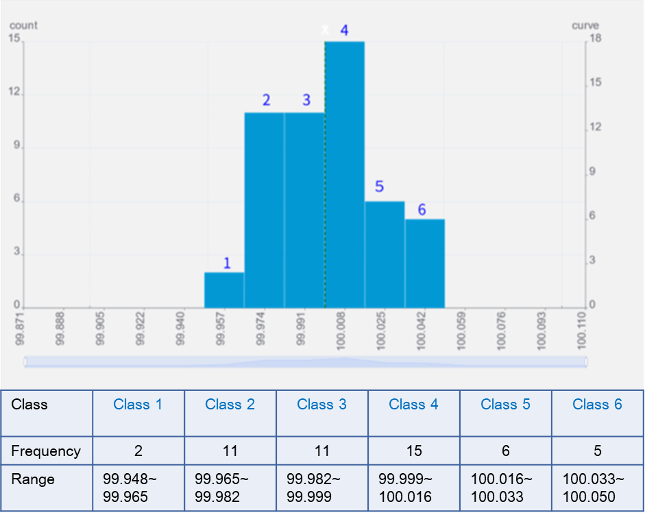
Classes (Bins)
- To draw a histogram, data must first be divided into classes (bins).
- When using tools like EXCEL, classes are usually determined automatically without the user having to worry about it.
- While there are multiple methods for binning, EXCEL and Python typically employ Scott’s normal reference rule.。
- Each class is divided at equal intervals, and the frequency (number of occurrences) within each class is counted.
| Class | Class 1 | Class 2 | Class 3 | Class 4 | Class 5 | Class 6 |
| Frequency | 2 | 11 | 11 | 15 | 6 | 5 |
| Range | 99.948~ 99.965 | 99.965~ 99.982 | 99.982~ 99.999 | 99.999~ 100.016 | 100.016~ 100.033 | 100.033~ 100.050 |
How to Plot a Histogram
- Each class's data is plotted as a single bar in a bar graph.
- The chart below is divided into 6 bars (classes).
*The example on the right uses Scott’s normal reference rule for calculation, but the formula has been slightly modified to improve graph legibility, so the number of classes may differ slightly from EXCEL.
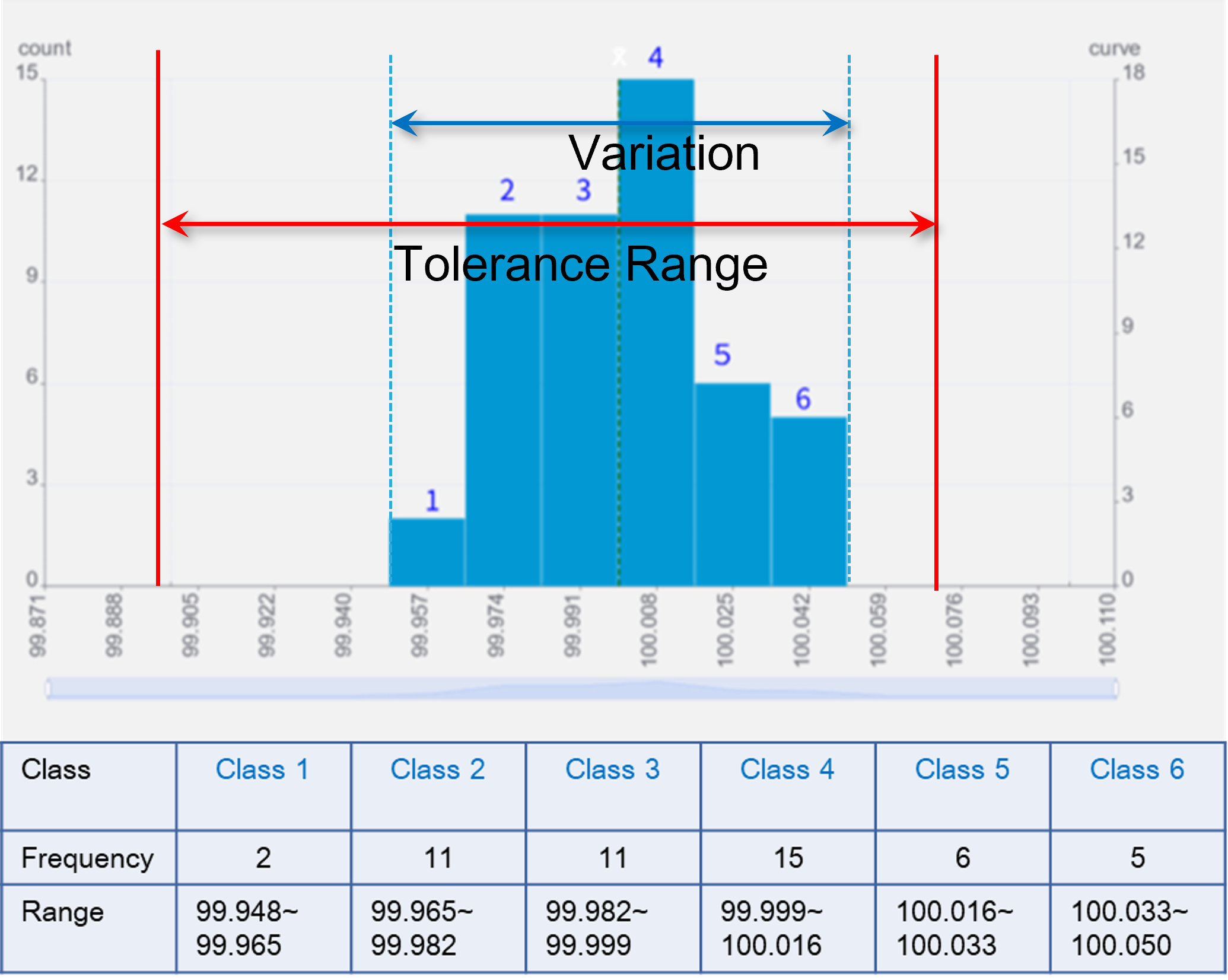
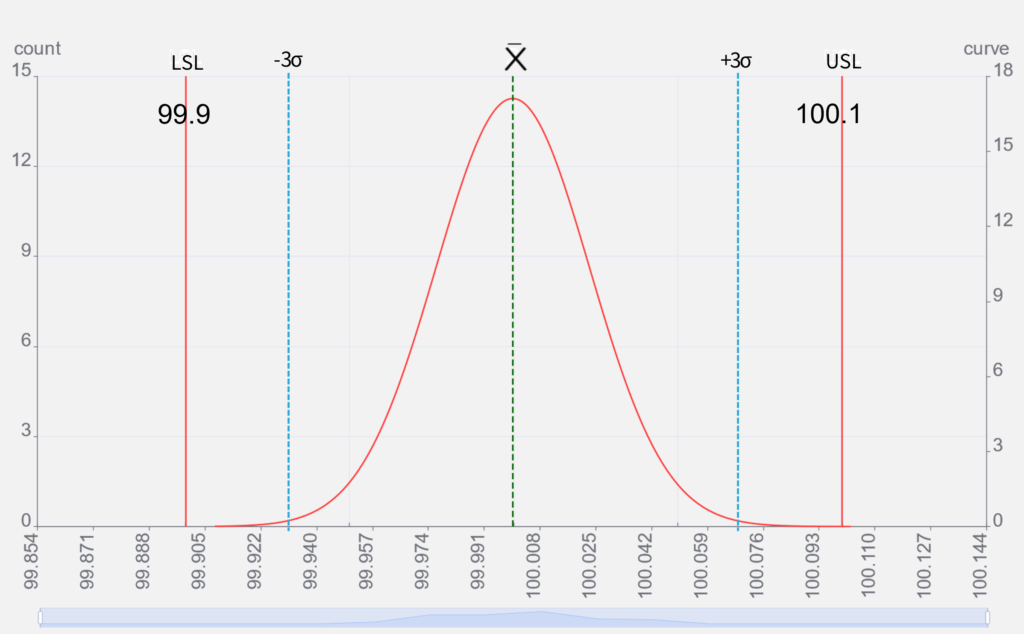
The graph on the right adds the following to the previous one:
- Upper Specification Limit (USL)
- Lower Specification Limit (LSL)
Comparing the width of the data variation with the tolerance range, all 50 data points are within tolerance, which appears favorable.
"What will the outcome be if we move to mass production in this state?"
Predicting this outcome is the role of process capability indices (Cp/Cpk), which serve as the criteria for deciding whether or not to begin mass production.
Distribution Curve
The graph on the right adds a:
- Distribution Curve
to the previous chart
This distribution curve is known as the Normal Distribution Curve (also called a Gaussian curve). It can be easily generated using spreadsheet software like EXCEL.
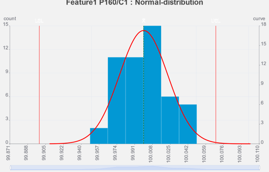
Properties of Normal Distribution
In general, data variation is said to follow a normal distribution curve. Therefore, we can predict that as more data is collected, the bar graph will grow to match the shape of the distribution curve.
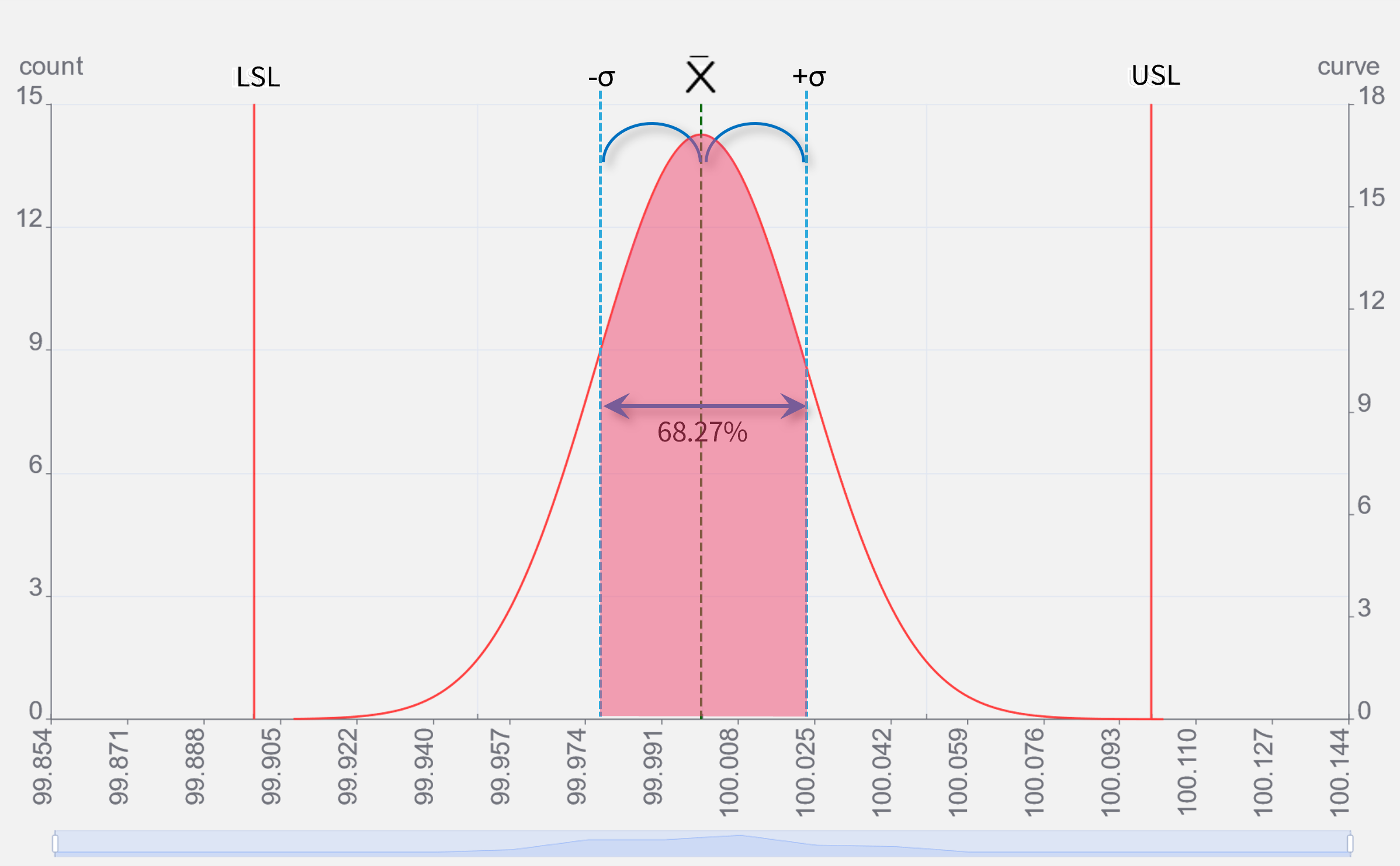
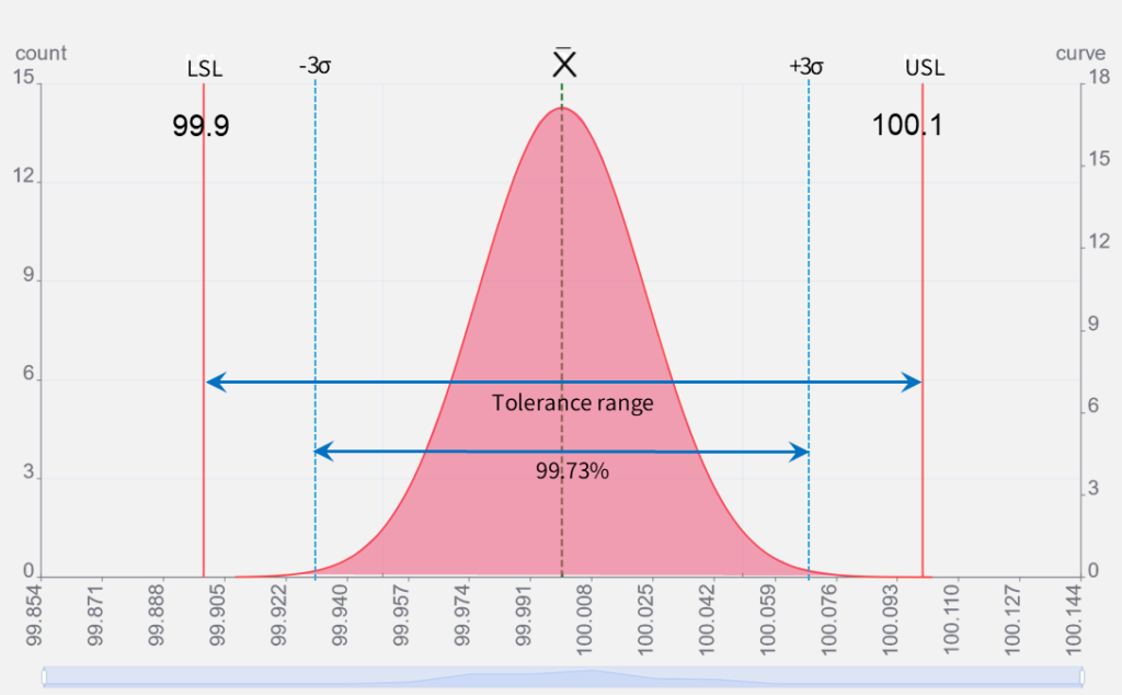
Meaning of σ (Sigma)
If the graph follows this distribution curve, we can predict the frequency of out-of-tolerance occurrences by comparing the distribution curve's width to the tolerance range.
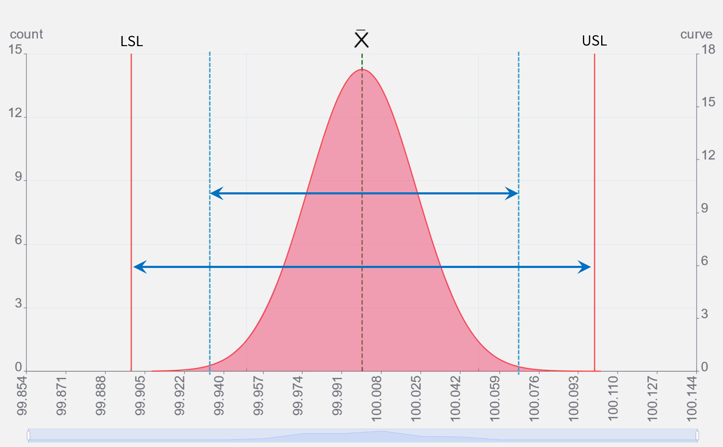
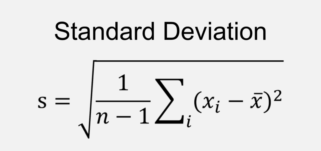
Calcuating σ
- The standard deviation σ can be calculated from the normal distribution curve.
- It is known that ±1σ (a width of 2) covers 68.27% of the area under the curve.
Meaning of 3σ
By simply multiplying σ by six, we can easily calculate almost the entire range (99.73%) of the distribution curve. This makes it a convenient benchmark for comparison with tolerances.
Why not use the 100% range?
Real-world data always contains outliers. If we compared the tolerance to the absolute maximum and minimum of all data, the range would include outliers caused by input errors or measurement equipment malfunctions. Therefore, we focus on the data excluding these extreme outliers.
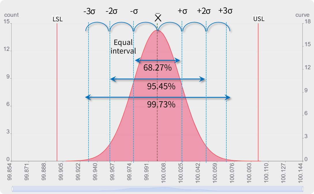
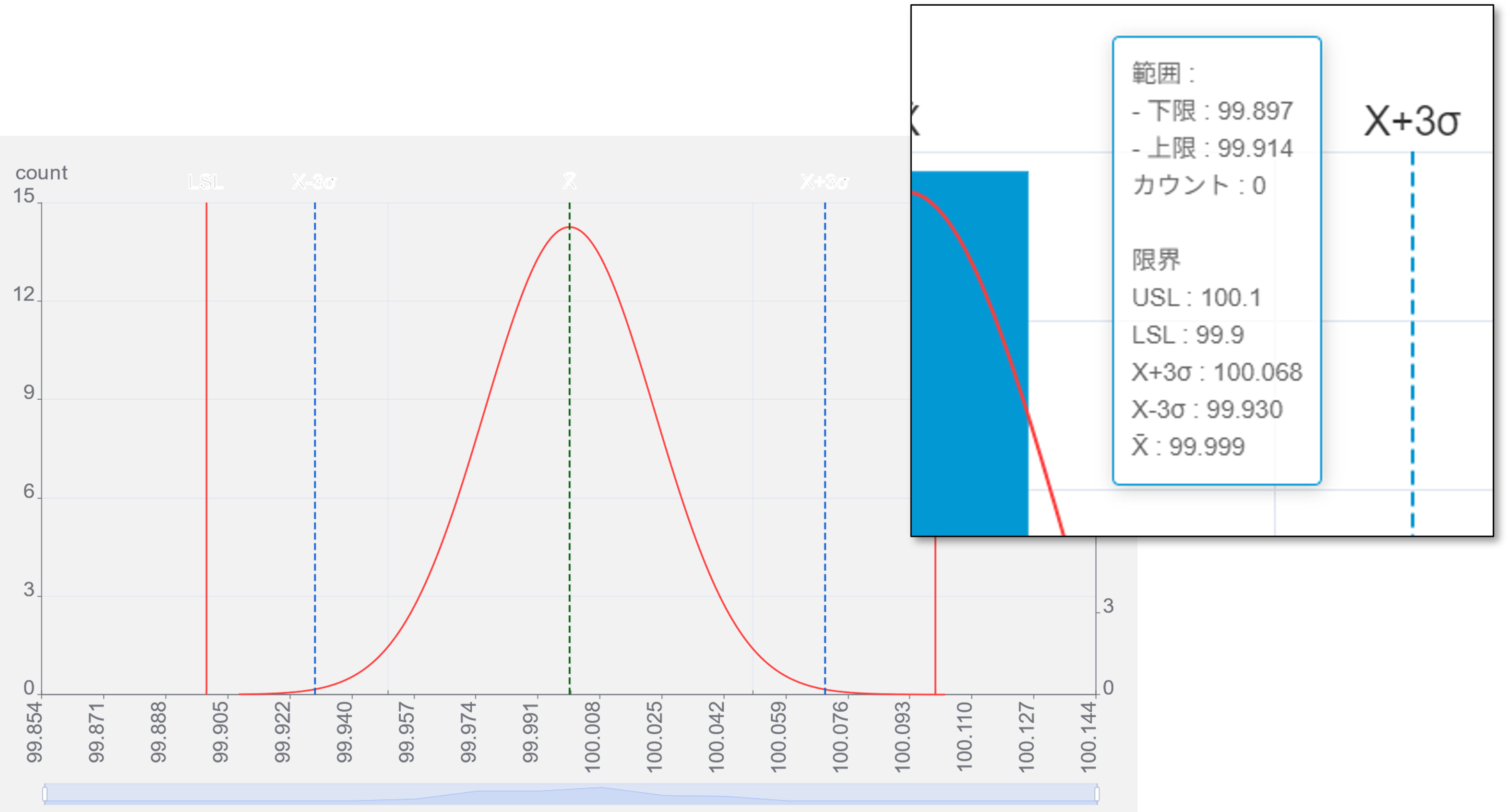
±3σ Range VS Tolerance Range
In this case, it is predicted that as data collection continues, almost all values will fall between 99.930 and 100.068. Statistically, if 1,000 data points are recorded, the probability of a data point appearing outside the ±3σ range is 2.7 out of 1,000—essentially 3 or fewer.
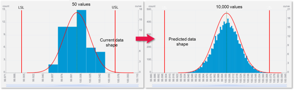
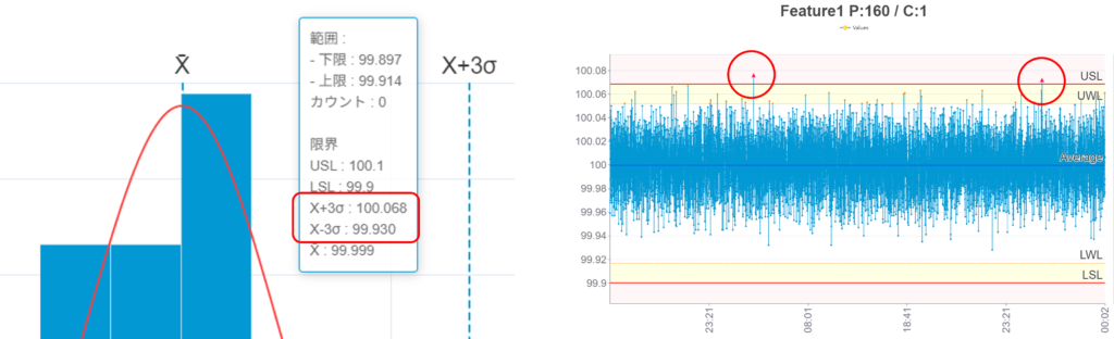
Prediction vs. Results
Based on the initial 50 data points, the predicted variation range was 99.930 to 100.068 (left chart). After observing up to 1,000 data points (right chart), only 2 points fell outside the ±3σ range, confirming that the results were largely as predicted.
CP
Calculating Cp
While we have been comparing the 6σ width with the tolerance width (USL - LSL), Cp and Cpk are the indices that express this comparison numerically.
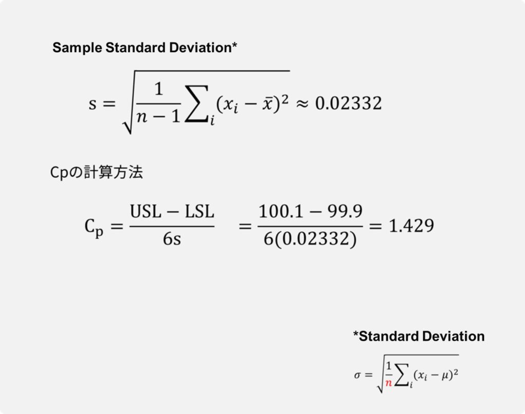
Calculation Method
- Calculate the sample standard deviation.
- Calculate Cp.
Meaning of Cp
Cp=1.429 can be intuitively understood as:
- "The tolerance range can fit approximately 1.4 variation ranges."
- "The tolerance range is approximately 1.4 times larger than the variation range."
Generally, a value of 1.33 or higher is considered good. Under stricter standards, passing thresholds may be set at 1.67 or 2.0.
Cp Summary
■
Cp is relative evaluation against the tolerance range.
■
Low Cp=Large variation (relative to tolerance)
■
Hight Cp=Small variation (relative to tolerance)
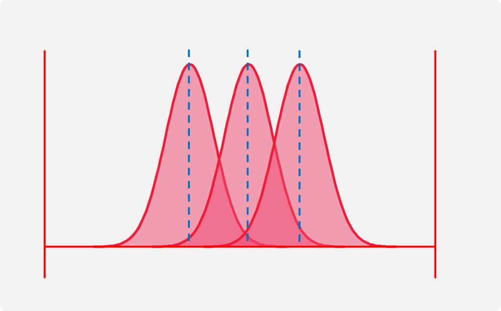
Properties of Cp
■
does not consider the position of the distribution.
●
The three histograms below all have the same Cp value.
■
The value of Cpk changes depending on the position of the distribution.
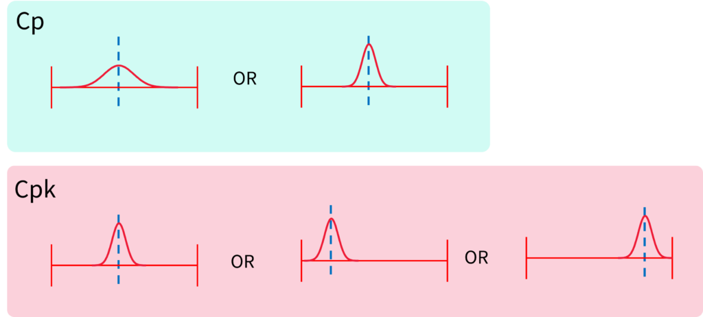
Cpk
■
Cp evaluates the width of the distribution (variation).
■
Cpk evaluates both the width and the "position" of the distribution.
Calculating Cpk
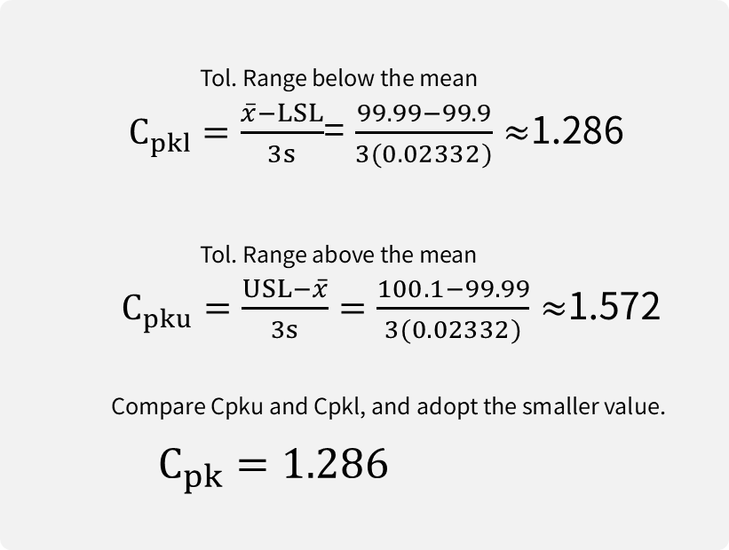
Cpk evaluates the distribution by splitting it into two parts: above the mean and below the mean.
We calculate Cpl(Lower) and Cpku(Upper) separately and adopt the smaller value as the Cpk.
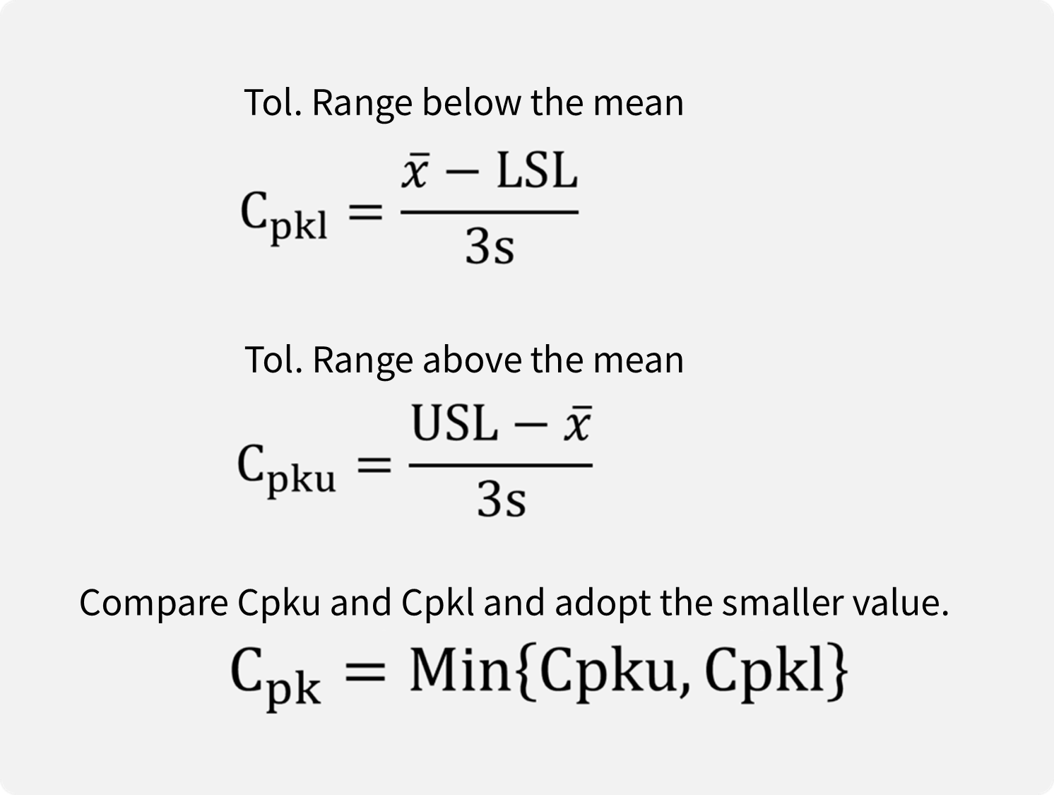
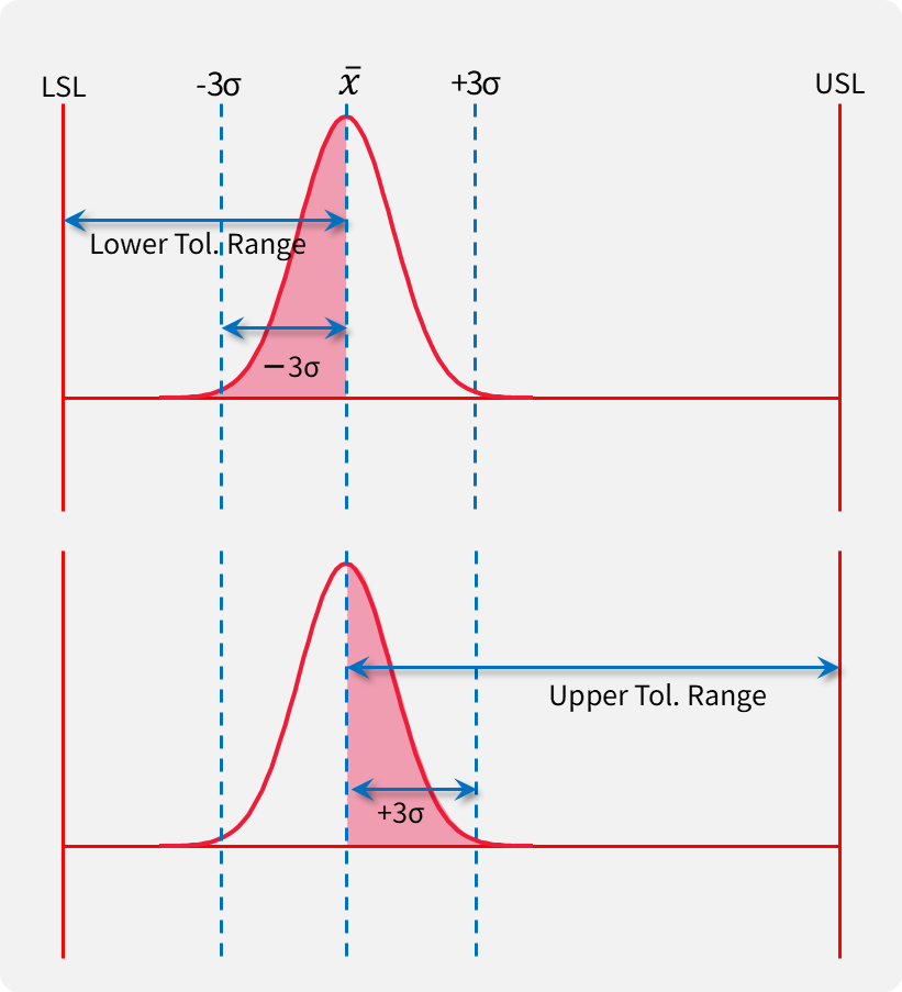
Let's look at an actual calculation.
From the Cp calculation, the standard deviation is 0.02332. Let's assume the mean (x bar) is 99.9.
Relationship with PPM
The defect rate in PPM (parts per million) can also be calculated from Cpk.
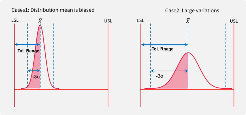
Properties of Cpk
There are two primary reasons why Cpk decreases (worsens):
■
Large variation
■
The mean position of the distribution is biased (off-center)
In both cases (or a combination of both), the difference in the numerator (x bar - LSL or USL - x bar) decreases relative to the denominator (3σ), resulting in a smaller Cpk value.
Cpk Summary
■
Cp/Cpk are relative evaluations against the tolerance ranges.

■
Small Cpk = Large variation, distribution center is biased toward either the LSL or USL, or both.

■
Large Cpk=Small variation, and the distribution center is not significantly biased.

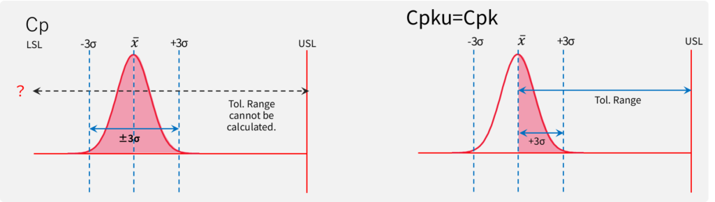
Case 1 where Cp cannot be evaluated: One-sided Specification
In the case of a one-sided specification limit, either the LSL or USL is missing, making it impossible to calculate Cp. Therefore, only Cpk is calculated.
■
For one-sided specifications, evaluate using Cpk only.
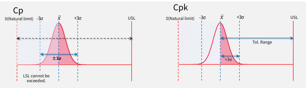
Case 2 where Cp cannot be evaluated: One-sided Tolerance (Natural Limit)
Geometric tolerances such as roundness, flatness, and perpendicularity involve one-sided tolerances where the LSL is naturally 0. Since both an LSL and USL technically exist, Cp can be calculated. However, no matter how much variation occurs, it is physically impossible to exceed the 0 limit (barring data entry errors). This type of boundary is called a Natural Limit. In such cases, the LSL represents the target value, so values close to the LSL direction are perfectly acceptable. Therefore, variation toward the LSL does not need to be considered. Consequently, only Cpk is calculated.
■
Variation toward a natural limit is not considered problematic since it cannot exceed the boundary.
■
Calculating Cp is not meaningful in these cases.
■
Calculate the half of the distribution that is NOT toward the natural limit and adopt it as Cpk.
Non-Normal Distribution
As explained previously, geometric tolerances like straightness often have a natural limit at the LSL. Such data only varies in the positive direction.
In reality, this type of data does not follow a normal distribution.
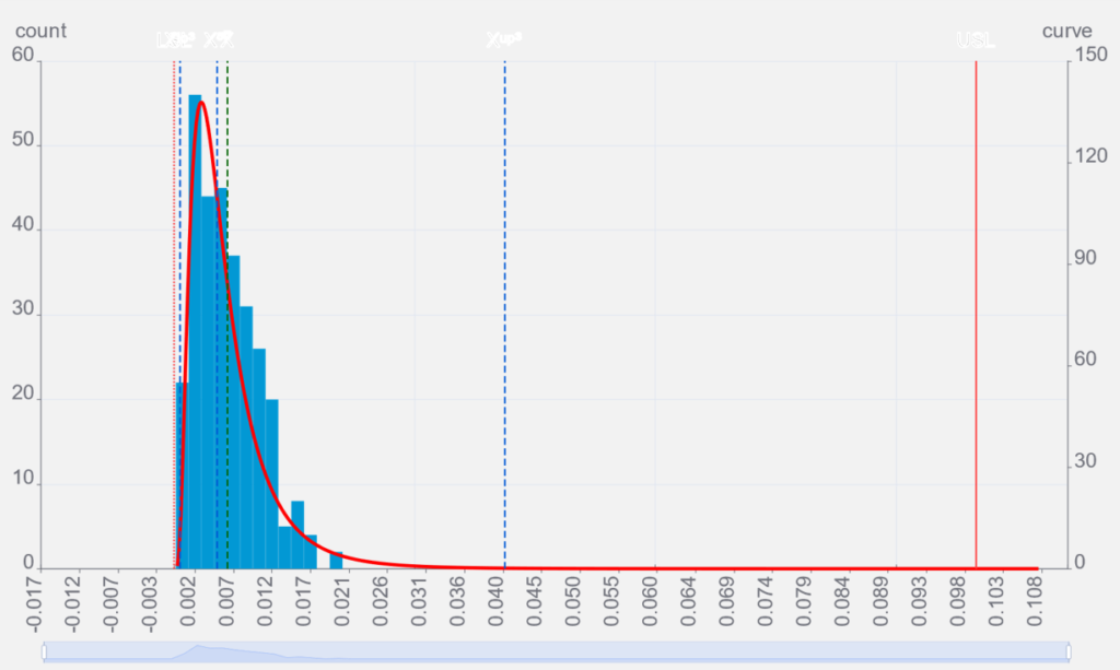
For non-normal distributions, process capability cannot be calculated using standard deviation as it is for normal distributions. The calculation methods for non-normal distributions are explained in Process Capability: Cp/Cpk No. 2.