Process Capability Calculation for Non-Normal Distributions
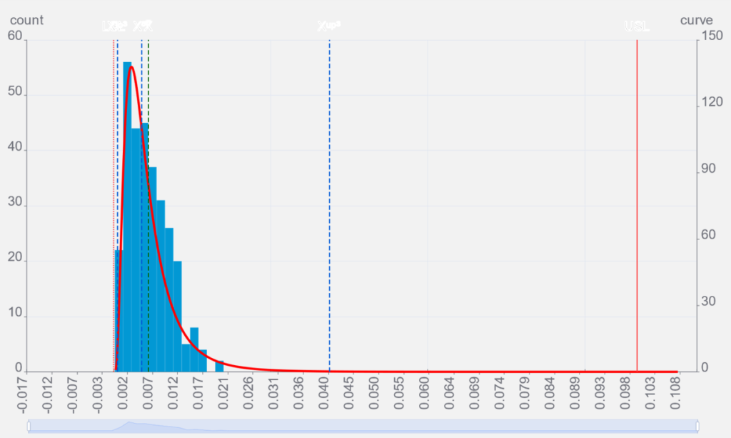
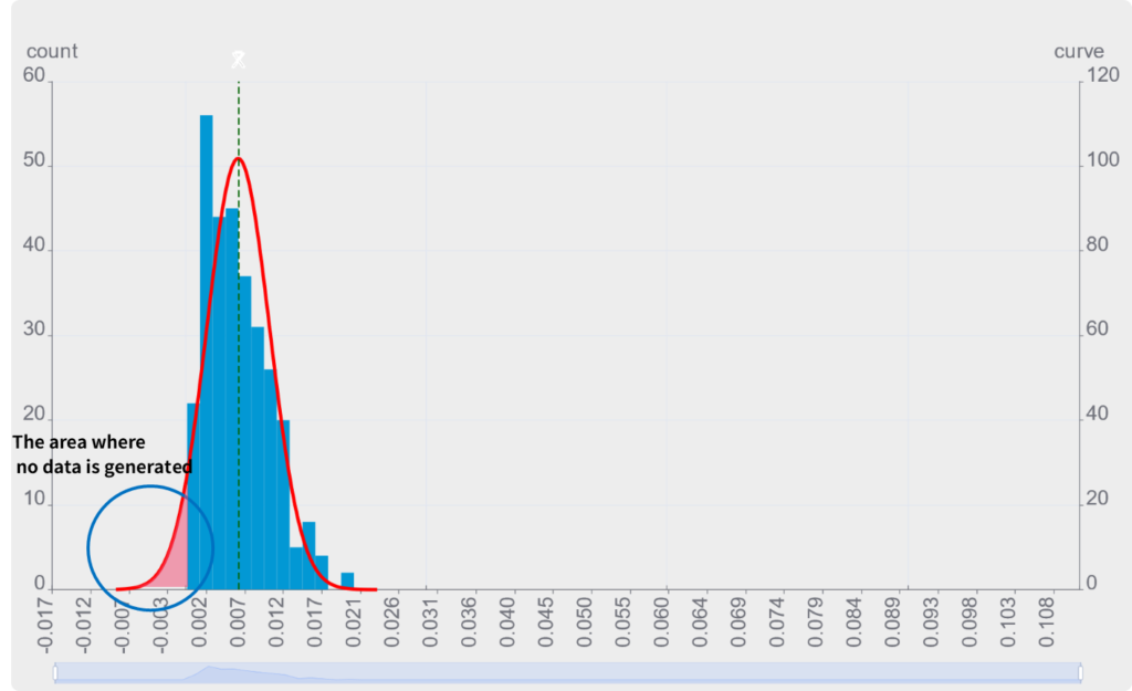
In Process Capability: Cp/Cpk No.1, we explained that for geometric tolerances such as straightness, the Lower Specification Limit (LSL) serves as a natural limit. Such data varies only in the positive direction.
In fact, the distribution of such data does not follow a normal distribution curve.
Impact of Non-Fitting Distribution Models
If you force a normal distribution model to calculate process capability for such data, the model will predict occurrences below zero—where data cannot exist in reality—leading to results that do not align with the actual situation.
Characteristics of Normal Distribution
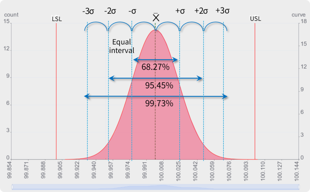
All process capability calculations discussed so far assume that the data follows a normal distribution. The normal distribution is a special case among many types of distribution curves, characterized by the ease with which process capability is determined using the standard deviation (σ). This is based on the premise that the intervals between 1σ, 2σ, and 3σ are equal.
Characteristics of Non-Normal Distribution
In the case of a non-normal distribution, the standard deviation (σ) used previously for process capability calculations cannot be applied directly.
■
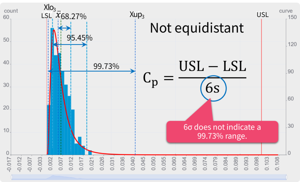
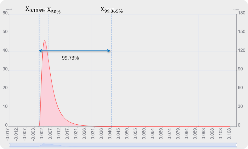
As shown below, in a non-normal distribution, even if you calculate the standard deviation,±3σ does not correspond to the 99.73% coverage range.
■
In a non-normal distribution, the intervals equivalent to 1σ, 2σ, and 3σ are not equidistant.
The Meaning of Process Capability Calculation
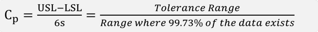
For non-normal distributions, process capability cannot be calculated using σ. However, let us reconsider the meaning of the process capability formula. The 6σ portion represents the variation range (the range where 99.73% of the data exists). In other words, if we can identify the positions equivalent to -3σ and +3σ indicating this 99.73% region without relying on the standard deviation, the formula remains valid.
Quantiles
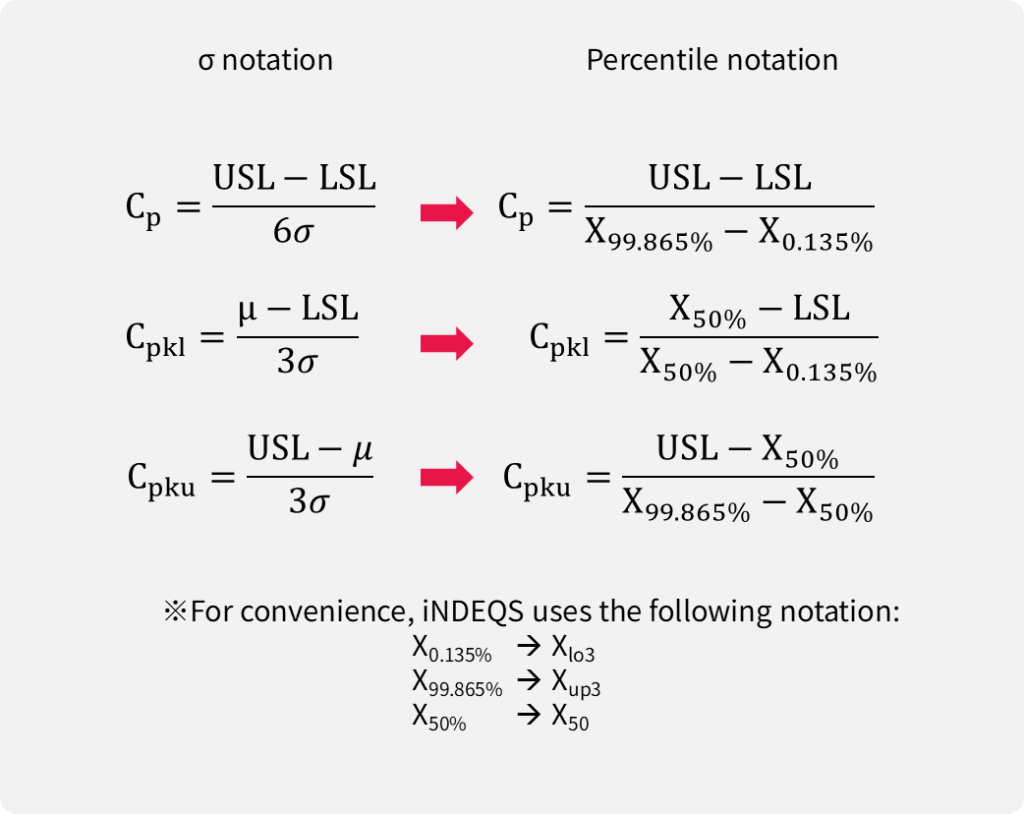
Even if you understand the underlying theory, calculating the range equivalent to 3σ for a non-normal distribution is no simple task. The iNDEQS software mathematically identifies the best-fit distribution model based on the "statistical estimation" methods outlined in ISO 22514-4. Using the selected model, the software performs quantile calculations in compliance with ISO 22514-2 to determine the 6σ equivalent range (99.73%)—specifically, the 0.135% and 99.865% quantiles1
Replacing with Percentile Notation
In the case of a non-normal distribution, the median is used instead of the mean (μ) because it is more robust to outliers. Therefore, you simply change from the mean (σ) to the median (percentile notation = X50%) and change the denominator to percentile notation. The basic formula Cp/Cpk holds true simply by swapping the numbers.
Necessity of Non-Normal Distribution Evaluation
In addition to natural limits, characteristics that appear normally distributed in the short term almost always become non-normal when evaluated over a long period.
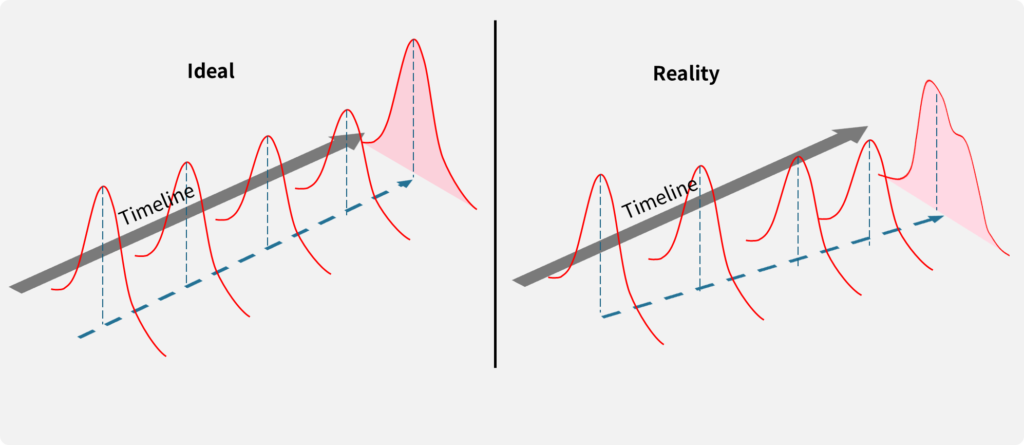
Factors of Process Variation
A process that is stable over a short period of time can fluctuate due to the "5M" factors: Man, Method, Material, Machine, and Milieu (Environment).
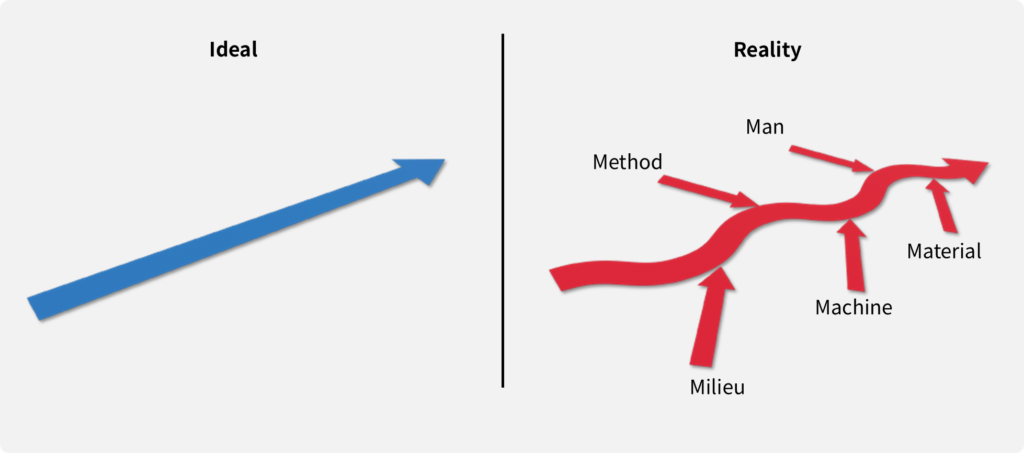
Strategies for Stability
For example, to make a process more stable, the following actions might be considered:
- Frequent machine adjustments
- Precise temperature control
- Frequent calibration of measuring instruments
- Extensive operator training
However, there are technical, temporal, and financial limits. Since we must perform process capability evaluations while maintaining the highest economic rationality, it is necessary to evaluate data as they are, regardless of whether they remain non-normally distributed.
Reasons for using Dedicated Statistical Software
For learning purposes, it can be done using EXCEL. However, most mass production uses dedicated software. The main reasons include:
- General spreadsheet software struggles with process capability prediction for non-normal data.
- Too many inspection characteristics to evaluate.
- Excel-based manual calculations are inadequate for handling process capability across a high volume of inspection characteristics.
- Multidimensional analysis using different data cuts (for each 5M factor) is possible.
- Spreadsheet software is unsuited for shifting between different data perspectives.
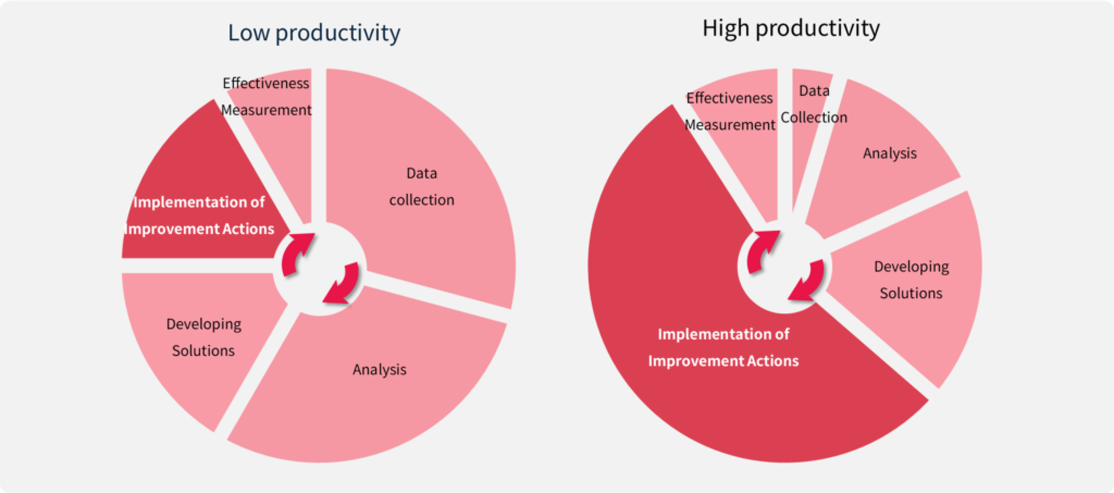
The greatest advantage of dedicated software is automation and speed. While collecting data, conducting analysis, and developing solutions are vital, in practice, there is no time to manually open general-purpose software, extract data for one's assigned process, and analyze it every time. A single manager may need to oversee hundreds or thousands of characteristics. If this task consumes too much time, it becomes impossible to respond to defects in a timely manner, and many defective products may be produced before the problem is even identified.
For analysis during process setup, we recommend using i-Analyzer, which allows for detailed conditional analysis. However, once the line is running, we use i-Board to eliminate tedious repetitive operations, automate analysis procedures that general-purpose tools struggle with, and enable real-time sharing of quality information across the entire process.
- Quantiles vary depending on the distribution model used to fit the data. iNDEQS automatically tests several candidate distribution models and calculates percentiles based on the curve that provides the best fit. ↩︎